Introducing Epidata v4

Epidata v0.4.0 (“v4” for short) launched on September 26, 2022, bringing about a major revision to how we store data served by the Epidata API. The changes prioritize fast access to the most up-to-date data while retaining the deep data revision history needed by researchers. The launch included a prototype of a modular data organization system intended to generalize across multiple pathogens, with stubs for more advanced and efficient timestamping and greater flexibility in data stratification.
In this post, we will discuss why these changes were needed, describe the new data architecture, and give a brief summary of how v4 performance compares to the previous version.
Motivation
This work was driven by the necessity to fix several specific deficiencies in the initial design of the covidcast table. As is often the case, these were somewhat easy to ignore at first, but soon became more pronounced over time. They can be grouped into three categories: 1) deficiencies affecting consumers of our API, 2) those affecting our ability to perform data ingestion/repairs and develop against the system, and 3) those affecting our ability to perform systems maintenance tasks efficiently.
1. Customer Affecting
- Slow analytics queries:
- Computing any kind of aggregate summaries in v3 was excessively expensive, with queries frequently requiring hours or even days to complete. Aggregate statistics and other analytics queries are needed in order to help determine the scope of outages (How many rows were added during the period when the bad code was live, and what range of time values were affected?) as well as quantify the impact of our dataset for project reports and proposals (How much data do we have from each of our different data sources? What is typical latency? How does latency behavior differ for different types of data sources?).
- Slow latest queries:
- Some data sources experience heavy revisions. The design of the v3 system required the database to scan all available issues of each matching reference date before it could identify the latest issue. The more revisions it needed to discard, the more time needed for the scan.
- COVIDcast Metadata:
- We compile a list of all COVIDcast-related sources and signals available in the API, along with basic summary statistics such as the dates they are available, their minimum and maximum values, and the geographic levels at which they are reported. This is made available here.
- The query to produce these aggregations was expensive in v3, requiring nearly five hours to run. Ideally we would like to update the metadata each hour when new data is added to the system.
2. Data Ingestion/Repair and Development
is_latestcolumn:- Because v3 recorded which row represented the most up-to-date value among a set of revisions using a flag, this flag had to be meticulously maintained to ensure that exactly one row for each (
source,signal,time_type,time_value,geo_type,geo_value) tuple had theis_latestflag set. This flag had to be unset when newer data was added, but left in place when older data was patched. System faults while data was being loaded could leave the records in an inconsistent state where two or more, zero, or the wrong rows had the flag set. Detecting problems with this flag was computationally expensive.
- Because v3 recorded which row represented the most up-to-date value among a set of revisions using a flag, this flag had to be meticulously maintained to ensure that exactly one row for each (
- Reduce repetition/normalize
- The v3 table included the full text of the source, signal, geographic type, and geographic value for each row, such that we were storing millions of copies of identical information for rows that shared the same (
source,signal,geo_type,geo_value). Since the duplicated information was also the most common selection criteria, the indexes took up a disproportionate amount of space on disk relative to the size of the base dataset.
- The v3 table included the full text of the source, signal, geographic type, and geographic value for each row, such that we were storing millions of copies of identical information for rows that shared the same (
3. Systems Maintenance
- Decrease backup/restore time:
- As our dataset grows, we incur ever increasing penalties to backing up and restoring our database. Frequent backups are key to maintaining reasonable disaster recovery goals. Fast restoration times are desirable so that we may both minimize disruptions associated with data or infrastructure disasters, as well as bring up development systems with full datasets for running experiments at scale.
System design
Our initial v3 schema was based on a single-table design. This worked well for a time. Each row represented a data point in its entirety, the most significant being:
The data source and signal, specifying the providing authority (“JHU” for example) and the type of data (like number of people vaccinated as a percent of the population, or the number of hospital beds occupied by covid patients).
The geographic type and a specific location (such as “state” & “Pennsylvania” or “county” & “Allegheny”).
The time type (either day or week) along with an actual numeric for the time value that the data corresponds to.
An issue date (the day this data was provided to us, as data is often re-issued to provide updates when entities may be slow to report, or when errors are corrected).
The value of the data itself (typically a number representing a count or percentage, which also includes (when available) sample size and standard error).
A small single-table design can be manageable, but our data set grew very quickly and challenges appeared. In particular, it became more difficult for the system to locate the most recent “issue” for each data point. Accessing such data is especially pertinent because it represents the most recent and accurate information that we have, and it accounts for 65 percent of the requests we receive. To ameliorate performance degradation, we added an additional column to flag the “latest issue” of data for each source, signal, time, and location. This helped but still left lingering concerns about speed. Also, adding this flag meant that we had to make sure it was appropriately updated whenever new data was issued. We had a few unfortunate events where this flag was not updated correctly, and the remedy can be quite time consuming.
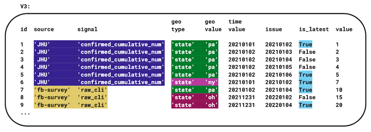
Fig 1: simplified diagram of v3 single-table design, with color coding marking areas improved in v4. Full v3 schema details available on GitHub.
Eventually we undertook the challenge of trying to improve our performance and reduce our resource usage – to come up with v4!
We chose to switch from MariaDB to Percona Server for MySQL for our database engine and management system. Both are variants of the free open source MySQL database, and both provide additional support and features on top of the base product. Percona offered us access to a more consistently developed drop-in replacement for MySQL, along with expertise and knowledge concentrated in both the open source community and Percona the company. Additionally, Percona Server for MySQL is a reliable target for monitoring with Percona’s PMM.
To reduce our data footprint and speed lookups, we took steps to “normalize” our database. This involved redefining our schema to move some columns out of the main table and into tables of their own, which we reference with “foreign key” columns instead. By arranging our data this way, the long and often-repeated text strings that name our sources and signals as well as the geographic locations we cover are only stored once each, and referred to by a number instead. The relatively short numbers take up much less space on disk compared to the text that they replace, and the database can optimize locating records by these numbers more easily than it can for text. We employ two of these dimension tables, one for source and signal, and one for geographic type and value. Using dimension tables efficiently requires JOIN operations when retrieving from the database. We avoided adding these slightly-more-complicated JOIN statements to many places in our code base by hiding them behind VIEWs – our VIEWs are a shortcut to the JOIN logic that make our new normalized tables look virtually indistinguishable from old monolithic table to our web server code.
We also added a “latest” table that includes a copy of just the issues that are most recent for all of our data points and removed the latest issue flag is_latest. Since this no longer relies on looking in our gigantic collection of all issues for data that is flagged as being the latest, we gained a significant improvement to query times. This is the data that drives our main website, so it is important for these operations to be fast for those browsing, and since we have so many visitors, it adds up to reduce our load significantly. The “latest table” simplifies our data management responsibilities compared to the “latest flag”, in that we don’t have to clear a flag from an old row (a previously “latest” issue of data) when a new “latest” row is added – instead we simply overwrite the old row in our latest table, and the database does this with great ease.
Additionally, the reduced size of the foreign keys compared to their text equivalents made it possible to include more indexes in our database that let it quickly find data based on different subsets of criteria. No matter how our users specify their requests, we have ways to look it up fast.
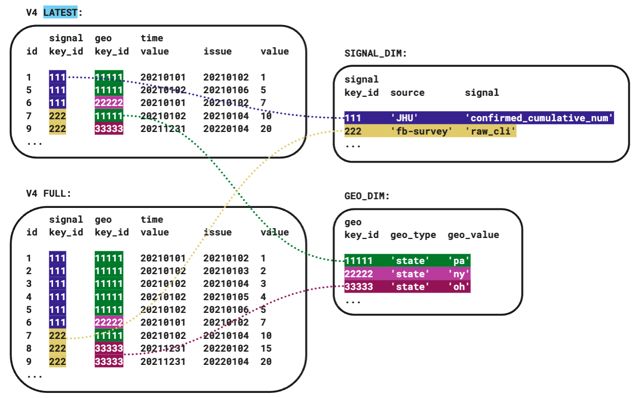
Fig 2: simplified diagram of v4 design, showing dimension tables with foreign key relationships and latest/full table scheme. Full v4 schema details available on GitHub.
Performance results
All performance figures were collected in an isolated QA environment. The core dataset was taken from a September, 2021 snapshot of the production Epidata database and used as-is for v3 experiments and converted to v4 format for v4 experiments. Performance experiments for v3 and v4 were both run on the same machine during dedicated time when nothing else was running. Input data for the “Adding new data” experiment was collected from data actually added to the production system in late May 2022. Input data for the query time experiments was sampled from a segment of actual query logs from July and August 2021, stratified by a generalized parameterized query template. Stratification ensured the samples were reasonably representative of actual traffic in terms of how many reference dates, regions, and signals are requested in a single query, as well as whether queries require the full data revision history or only the most recent issue of each reference date. Additional details about query log sampling will be included in a future post.
Overall, the v4 system improves Epidata performance for adding new data and substantially improves performance for querying the most up-to-date figures. Storage performance is the same, although we suspect we could improve this by removing an index or two without much impact on query performance. Query performance for queries that must touch the data revision history is worse, but not by much; performance should still be adequate for most research use cases (please do get in touch if this is not the case for you).
| Metric | v4 performance relative to v3 |
|---|---|
| Disk footprint | same |
| Adding new data | 30% faster |
| Querying latest data, i.e. the most recent issue of any reference date | 96% faster |
| Querying historical data, e.g. for as-of, issue, or lag queries | 120% slower |
The largest factor in the query time improvements for latest data is a reduction in the frequency and severity of long-running queries. In v3, over seven hundred queries required over ten seconds to compute, and the longest-running query took twelve minutes; in v4 only three queries needed more than ten seconds and no query took more than twenty-one seconds.
| Query time (seconds) | Latest | Historical | ||
|---|---|---|---|---|
| Percentile | v3 | v4 | v3 | v4 |
| 0th (minimum) | 0.005 | 0.005 | 0.005 | 0 .005 |
| 25th | 0.007 | 0.006 | 0.006 | 0.007 |
| 50th (median) | 0.009 | 0.008 | 0.007 | 0.008 |
| 75th | 0.058 | 0.017 | 0.012 | 0.023 |
| 100th (maximum) | 739.332 | 20.069 | 17.121 | 15.997 |
For historical data, long-running queries were more frequent in v4 than in v3, but not more severe. In v3, only 8 queries required more than one second to compute, and the longest-running query took seventeen seconds; in v4 over two hundred queries needed more than one second, but the max query time was sixteen seconds.
The empirical cumulative distribution functions for query times in the latest and historical datasets shows both of these effects in greater detail.
| Long-running queries (counts) | Latest (of 37,396) | Historical (of 19,359) | ||
|---|---|---|---|---|
| Queries slower than | v3 | v4 | v3 | v4 |
| 1 second | 2734 | 17 | 8 | 228 |
| 10 seconds | 706 | 3 | 1 | 1 |
| 100 seconds | 3 | 0 | 0 | 0 |
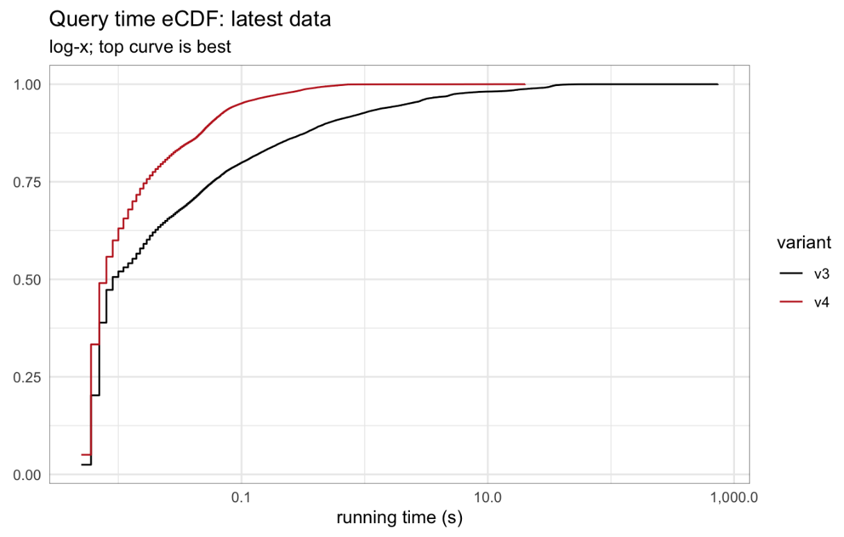
Fig 3: Empirical cumulative distribution functions for query times, latest data
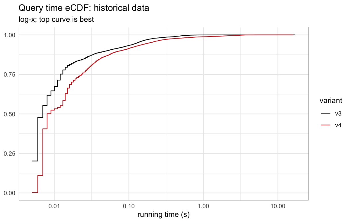
Fig 4: Empirical cumulative distribution functions for query times, historical data
If we compare the running time in each system for each query, we can get a more precise picture of whether and how times improve or worsen between the two systems. For queries of latest data, the vast majority of queries are faster in v4, but a few are slower, sometimes by more than 10x. For queries of historical data, v4 and v3 query time are typically similar, with a couple clouds of slower query times in v4.
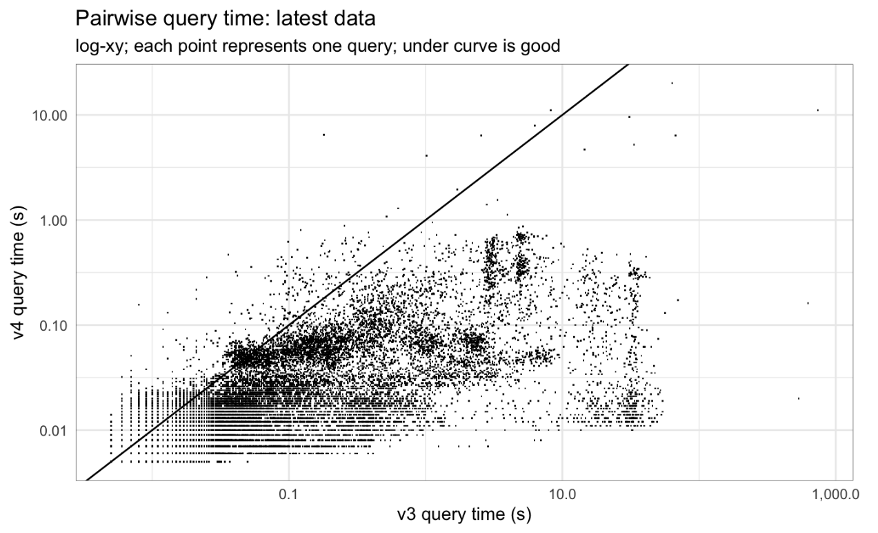
Fig 5: Pairwise query time, latest data
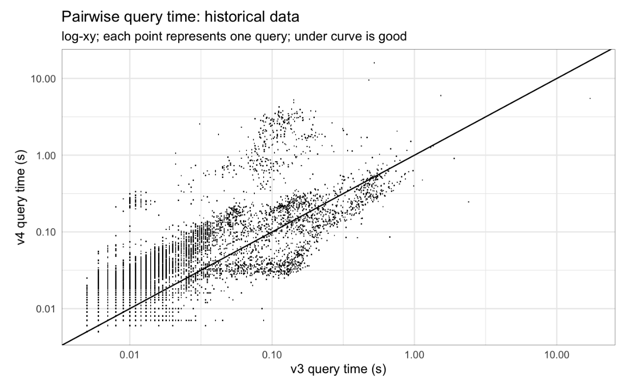
Fig 6: Pairwise query time, historical data
Conclusion
Epidata v4 represents an enormous and necessary effort in developing scalable access to versioned time series data. We’re excited to continue improving in this space! We have plans for:
- Realizing the timestamp stubs - taking advantage of database optimizations for datetime data, making it possible to track multiple updates each day or reference period, and accurately representing unusual reference periods (such as HHS Friday-Thursday weeks)
- Realizing the stratification stubs - permitting support for age, demographic, serotype, and other data splits
- Bringing up an influenza schema - transferring what we’ve learned from covid about geotemporally-detailed epidemic surveillance tracking, and proving the modular capabilities of the new system


